| Brief Description | |
|---|---|
|
Files: \examples\Processing\HDR_ImageComposition\ExposureFusion\ExposureFusion.vad |
 |
|
Default Platform: mE5-MA-VCL |
|
|
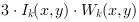
Short Description An image composition from up to 16 images with different exposure times to one image showing details and contrasts over complete image without over- and under exposed pixels. This example is a simple alternative to High Dynamic Range Imaging. |
|
Exposure fusion combines images with different exposure times to one image. In this resulting image under- and over exposed pixels are prevented and details are fully conserved. The aim of exposure fusion is similar to High Dynamic Range Imaging (see section and ), but in contrast to this method, the dynamic range of luminosity of the acquired images is not extended. Exposure fusion simply takes the best parts of the images of the sequence and combines them in one result image. Exposure fusion is easier to handle for the user, as he does not need to know the exposure times of the images acquired. The quality of the resulting image is slightly worse than with the algorithms of HDRI. In the following the exposure fusion algorithm, which is implemented in "ExposureFusion.vad" is introduced.
The exposure fusion algorithm according to [Mer07] combines images
of a sequence with length N with a weighted blending to a result image
 :
:
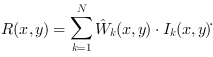
Here  is the weighting for each color component
red, green and blue
is the weighting for each color component
red, green and blue  of a pixel at position
 in the k-th image of the sequence with
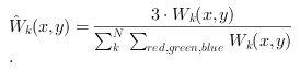
 is a weighting function, which is dependent on the pixel value
at position
is a weighting function, which is dependent on the pixel value
at position  and is a measure for the well-exposedness of this pixel.
In "ExposureFusion.vad"
and is a measure for the well-exposedness of this pixel.
In "ExposureFusion.vad"  is a linear function up to the pixel value of
127. For pixel values from 128 to 255,
is a linear function up to the pixel value of
127. For pixel values from 128 to 255,  is set to 127.
In dependence on his requirements the user easily can change this weighting function, as described in section
e.g. according to [Mer07].
Quality measures like contrast or saturation (see [Mer07]) are not implemented in this reference design.
In eq. 45 the sum over the color components red, green and blue in the denominator prevents, that a pixel
is set to 127.
In dependence on his requirements the user easily can change this weighting function, as described in section
e.g. according to [Mer07].
Quality measures like contrast or saturation (see [Mer07]) are not implemented in this reference design.
In eq. 45 the sum over the color components red, green and blue in the denominator prevents, that a pixel
 in the result image looses the color information of the original
images.
in the result image looses the color information of the original
images.
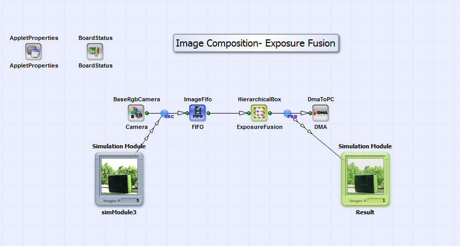
In Fig. 356 the basic design structure of "ExposureFusion.vad" is shown.
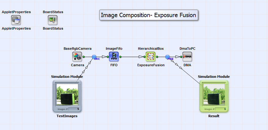
The images of a sequence from an rgb camera in Camera link base configuration are combined to one result image according to the algorithm in eq. 44 in the HierachicalBox ExposureFusion. For simulation purpose please load up to 16 images of maximum dimensions of 1024x1024 pixels to the simulation source TestImages. The order of the images with respect to their exposure times is not of importance! With "right-mouse-click" on box ExposureFusion you can set the image sequence length and the image dimensions of the input images. The maximum number of images is 16 and the maximum image dimensions are 1024x1024 pixels. The output image is sent via DMA to PC. In Fig. 357 the content of the HierarchicalBox ExposureFusion is shown.
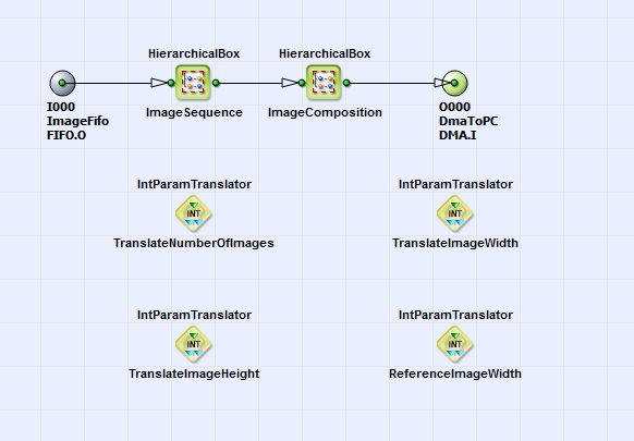
In the box ImageSequence the images from the sequence are combined to one large image. The pixels at position
 from the images are positioned as neighbors. In the box
ImageComposition the exposure fusion algorithm according to eq. 44 is implemented.
You can see its content in Fig. 358.
from the images are positioned as neighbors. In the box
ImageComposition the exposure fusion algorithm according to eq. 44 is implemented.
You can see its content in Fig. 358.
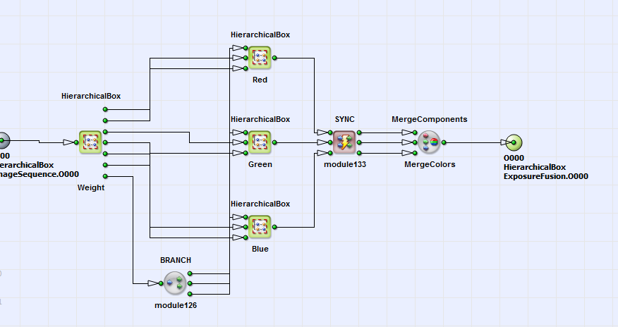
In box 重量 the weighting function  (see. eq. 45) in dependence of the pixel value is implemented for each color component. You can see the content of box
重量 in Fig. 359.
(see. eq. 45) in dependence of the pixel value is implemented for each color component. You can see the content of box
重量 in Fig. 359.
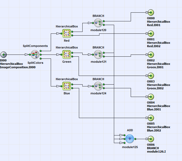
The weighting functions for each color component from boxes
红色, 绿色 and 蓝色 are summed up, according to eq. 45.
In Fig. 360 you can see the weighting function
 for the color red.
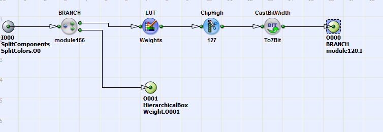
Up to a pixel value of 127 the function is linear. From pixels values 128 to 255,
 is set to 127.
The lookup table operator LUT_Weights allows the user to adapt the weighting function easily to his requirements. Also changing the parameters for the
ClipHigh and CastBitWidth operators (or even deleting them) gives the user this possibility. Coming back to the content of box
ImageComposition. Here according to eq.44
the pixel values
is set to 127.
The lookup table operator LUT_Weights allows the user to adapt the weighting function easily to his requirements. Also changing the parameters for the
ClipHigh and CastBitWidth operators (or even deleting them) gives the user this possibility. Coming back to the content of box
ImageComposition. Here according to eq.44
the pixel values  for the color components red, green and blue are
multiplied with the weighting function
for the color components red, green and blue are
multiplied with the weighting function  and with a constant
Const of value 3 in the boxes 红色, 绿色 and 蓝色. You can see the content of box
红色 in Fig. 361.
and with a constant
Const of value 3 in the boxes 红色, 绿色 and 蓝色. You can see the content of box
红色 in Fig. 361.
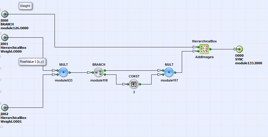
Here 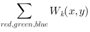 is summed up for all images.
 is then
divided by
is then
divided by 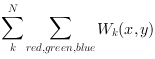 according to eq.
45. Finally the color components are merged together (see Fig.
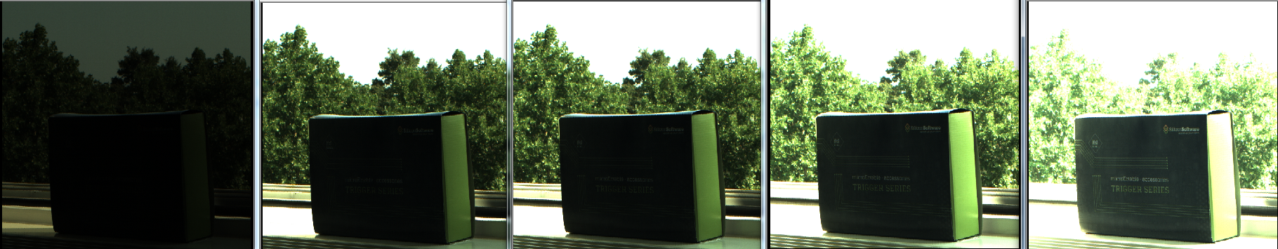
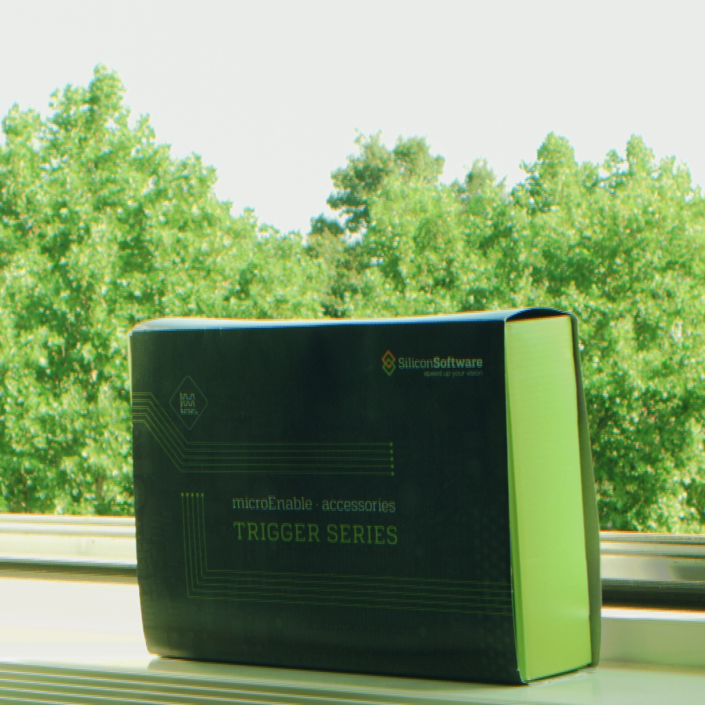
358) and the output image is sent to PC. In Fig. 362
you can see 5 example input images with the result image in Fig. 363. The result image has no under- and over exposed pixels and
details are conserved.
according to eq.
45. Finally the color components are merged together (see Fig.
358) and the output image is sent to PC. In Fig. 362
you can see 5 example input images with the result image in Fig. 363. The result image has no under- and over exposed pixels and
details are conserved.