VisualApplets provides powerful, functional simulation features for simulating designs. You can use simulation for a first test of the implemented image processing algorithm, and for its verification. You can start a simulation directly after editing the design without the need to build a *.hap file.
The simulation in VisualApplets is functional, i.e., it emulates the behavior of the hardware implementation. This makes it very fast compared to low level simulations. A side effect of the functional simulation is that timing is not considered. The simulation behavior of operators is 100% equal to the image processing of the final applet on real hardware.
To simulate the behavior of a design in VisualApplets, two kinds of simulation elements are provided:
-
simulation sources, and
-
simulation probes.
Simulation sources are used for data input. You can load one image or a whole image sequence into a simulation source (from image files). You can place one simulation source or one simulation probe at any link in your design. Thus, data transport along those links is overwritten by the connected source module or inspected by the respective probe module.
![[Note]](../common/images/admon/note.png) |
Note |
|---|---|
|
Some operators can function as an image source, too; e.g., operator CreateBlankImage. |
You can save the resulting images of the simulation probes to image files.
Due to visualization optimizations, the VisualApplets simulation is based on 2D images.
Nevertheless, you can also simulate if the link the simulation source is connected to is 0D (stream of pixels), 1D (stream of lines), or 2D (stream of frames), as long as the simulation source contains at least one 2D image (see 'Image Protocols, Image Dimensions and Data Structure').
Simulation has the following limitations:
-
The simulation of the SIGNAL image protocols is not possible. This is so, because the simulation of the SIGNAL image protocols emulates the functionality, but not the timing of a design. However for simulation of the SIGNAL image protocols, it would be necessary to simulate the timing, too.
-
The simulation of the 0D image protocol is limited to exactly one simulation step. This is so, because for simulation all pixel data of one source is aggregated to a single 2D frame. However, subsequent steps can be simulated for the remaining design, but operators generating 0D content will only emit data once during the first step.
-
The operator PseudoRandomNumberGen does not return the same result in a simulation as on the hardware. This is so, because the operator is non-deterministic. This exceptions is also described at Operator Reference.
-
The operator Blob Analysis 1D does not return the same result in a simulation as on the hardware. This is so, because the operator has the port FlushI, but as the flush is asynchronous to the image data, it cannot be simulated to reflect the same behavior as in hardware. This exception is also described at Operator Reference.
-
BMPsandTIFFswith indexed color palette are not supported.
The following image formats are supported for simulation in VisualApplets for source images as well as for saving the output images:
- Bitmap
-
BMP1 bit black/white (row length has to be a multiple of 8)BMP8 bit grayBMP24 bit (R8 G8 B8) sRGB color spaceCompression like RLE is not supported.
- TIFF (Tagged Image File Format)/TIF
-
TIFF1 bit black/white (row length has to be a multiple of 8)TIFF8 bit grayTIFF24 bit color sRGB color spaceTIFF48 bit color sRRB color spaceCompression: None, LZW, or PackBits
- JPEG/JPG
- PNG
- GIF
- PSD
Additionally, the following formats are supported as source images:
-
SVG
-
XCF
-
RAW
-
RSD (SiSoRawSimulationData)
|
Limitations |
|---|---|
|
|
Simulating image data processing in your design comprises the following steps:
-
Inserting the simulation sources and probes you need into your design.
-
Loading the image file(s) you want to use for simulation to your simulation source(s).
-
Optimizing your image input via parameters, such as pixel merge and pixel alignment.
-
Setting the number of processing cycles for the simulation in the main simulation window and starting the simulation.
-
Evaluating the simulation results.
-
Saving the simulation results.
In the following sections, these steps are be described in detail.
To prepare a simulation, you must first insert your simulation source(s) and probe(s) into your design:
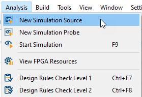
-
From the main menu, select → or use the corresponding icons in the toolbar to insert your source(s) and probe(s) into the current design window.
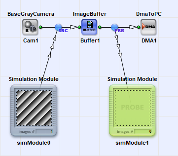
Simulation sources and simulation probes are both displayed as small image frames with a magnetic anchor:
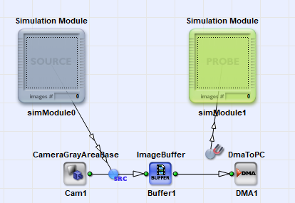
-
Use the anchor to connect the source or probe to a link in the design. You can easily distinguish simulation sources from simulation probes as sources are of gray, probes of green color.
-
Use drag and drop to position your source(s) and probe(s).
-
Use drag and drop to connect your source(s) and probe(s) to links in your design. If the anchor icon changes to blue, the connection is valid.
![[Caution]](../common/images/admon/caution.png) |
Connecting Simulation Sources and Probes to a Link Transporting Kernels or Signals |
|---|---|
|
You can connect a simulation source to a link that transports kernels, but the simulation source needs to provide exactly one input image per kernel. You can connect a simulation probe to a link that transports signals, but this simulation probe then doesn't provide any data. |
In the , you can load test images or test image sequences and make them available for simulation.
At first, let’s have a quick look at the .
-
To open the , double-click a source in your design.
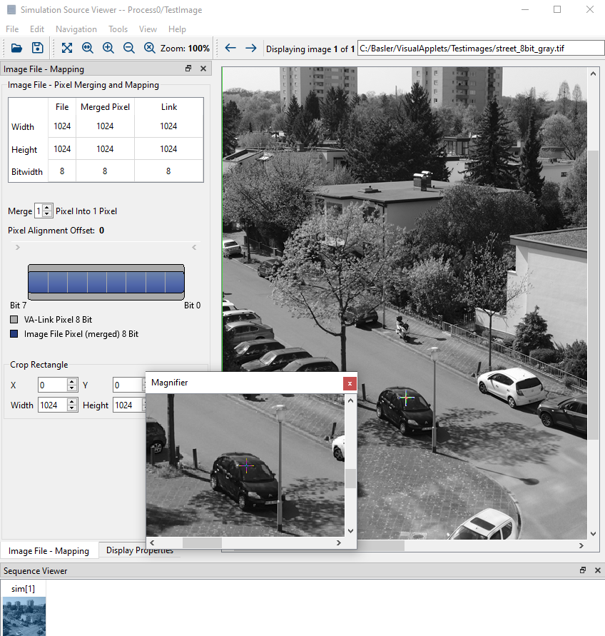
The opens up:
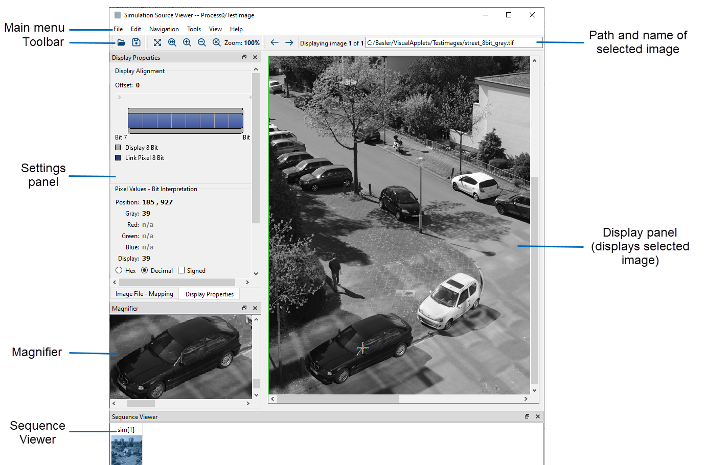
Directly under the menu, you find the toolbars. The icons of the toolbars offer the following options (left to right):
-
 File toolbar for opening and saving image files.
-
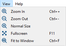
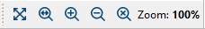 View toolbar offering different options for image
display. These are the same as the first options of the View menu:
View toolbar offering different options for image
display. These are the same as the first options of the View menu:
-
 The arrows for navigating through image
sequences.
The arrows for navigating through image
sequences.
-
 Display of details on the image currently visible in
the display panel of the main viewer window (and magnifier): Displays the
position of the image in the image sequence loaded to the simulator, and the
path to the image file
Display of details on the image currently visible in
the display panel of the main viewer window (and magnifier): Displays the
position of the image in the image sequence loaded to the simulator, and the
path to the image file
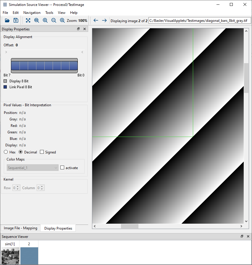
On the left hand side, you have the settings panel with two tabs:
- Image File – Mapping
-
Here, you can adjust the settings for simulation, e.g. enter a value for pixel merge, or define the offset for pixel alignment.
- Display Properties
-
Here, you can define the settings for displaying the test images on your own screen. Due to the fact, that monitors always use 8 bit color display, at times you have to decide which part of a pixel you want to see on screen for evaluating your test images. None of the settings you define under have influence on the simulation or its results.
In addition, you find here the color values of a selected pixel listed, together with the display value. The display value is the mapped value for display on the user monitor.
On the right hand side, you have the display panel displaying the image currently selected.
You can zoom in and out on the image displayed in the display channel by either using the corresponding icons in the toolbar, or by using CTRL+MouseWheelUp to zoom in and CTRL+MouseWheelDown to zoom out.
If you choose a very high zooming factor, a pixel grid is displayed for better orientation and hex/dec values per pixel are displayed.
On the bottom of the simulation viewer, you have another panel: This is the . If you use more than one image in a source, here you can see all images of the image sequence, make changes to the image order of the sequence, or select an image for display in the display panel and magnifier.
The is actually a second window of the which you can easily loosen from the main window via drag & drop. The always shows the same image as is displayed in the display panel of the main . Its pointer is always in the center of the window and positioned exactly on the pixel you point at in the display panel. The great advantage of the window is that you can display a selection of the image with a completely different zooming factor:
If you want to change the zooming factor of the :
-
Activate the → window.
-
Use CTRL+MouseWheelUp to zoom in and CTRL+MouseWheelDown to zoom out.
If you choose a very high zooming factor, a pixel grid is displayed for better orientation.
To load test images or test image sequences into your source,
-
Open the by double-clicking the source in your design.
-
From the main menu of the , select → or click the corresponding icon in the toolbar. In the following dialog, select the simulation input image file and click .
|
Note |
|---|---|
|
You find some useful test images in the VisualApplets installation folder
under |
![[Tip]](../common/images/admon/tip.png) |
提示 |
|---|---|
|
Alternatively, you can simply drag & drop image files either from your Windows Explorer into the viewer, or from your Windows Explorer onto the source in your diagram. |
The input image is now displayed in the .
After closing the , you see a thumbnail of the image in the preview frame of the corresponding source:
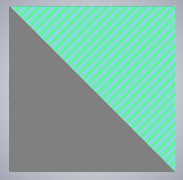
As soon as you connect a source to a link, the source takes over the parameter settings of the link (such as maximal image dimension, bit width, and color format). If you load an image that is bigger than the maximal image dimension of the link, a green rectangle is displayed on the image, enclosing the part of the image that will be used for simulation:
|
Convert your Images |
|---|---|
|
It is not possible to load a color picture on a one-channel gray link and vice versa. If your test image does not fit the properties of the link the source is connected to, you need to convert the image. Use any image processing program that offers the necessary functions to convert your test image. Use an image format supported by VisualApplets. For information on supported image formats, see 'Supported Image Formats'. |
As soon as you load a new image to the source, the image shows up in the display panel of the and is added to the image sequence of your source. You can see all images of your image sequence in the , which is located at the bottom of the .
Only the selected image displayed in the display channel is stored in the RAM of the computer. The other images of the sequence are loaded into the RAM when necessary. Thus, loading long image sequences onto a source has nearly no impact on RAM usage.
If you load an image sequence, you can change the order of images after load. In the , use drag & drop to position an image to where you want it to be in the sequence.
You can easily delete one or more images of a sequence:
-
Press CTRL and select the images you want to delete.
-
Press DEL or select from the menu → .
In the , indicates the image that is being simulated during the next simulation step. You can reset to the first image of the sequence in the Simulation dialog by clicking the button. If you want to know more about simulation steps and reset, see 'Setting the Number of Processing Cycles and Starting the Simulation'. The simulation order is not influenced by the image currently displayed in the display panel.
![sim[x] Indicates the Image that Is Simulated in a Sequence](../../images/user-manual/simulation/sim[x].PNG)
If you change the image properties by mapping (see 'Image File Mapping '), the thumbnails are not refreshed automatically. By default, the displays the thumbnails of the original images.
You have two possibilities to adapt the thumbnail display. From the menu, select either
-
→ to get a preview on how your images will look after applying the current mapping settings in a simulation, or
-
→ to have thumbnails displayed that reflect the current look of your images.
You can now optimize your image input via parameters. All parameters are displayed in the .
On each pixel in the display panel, actually two crosshair cursors are displayed If you can’t see the two crosshair cursors, zoom in on the picture in the display panel:
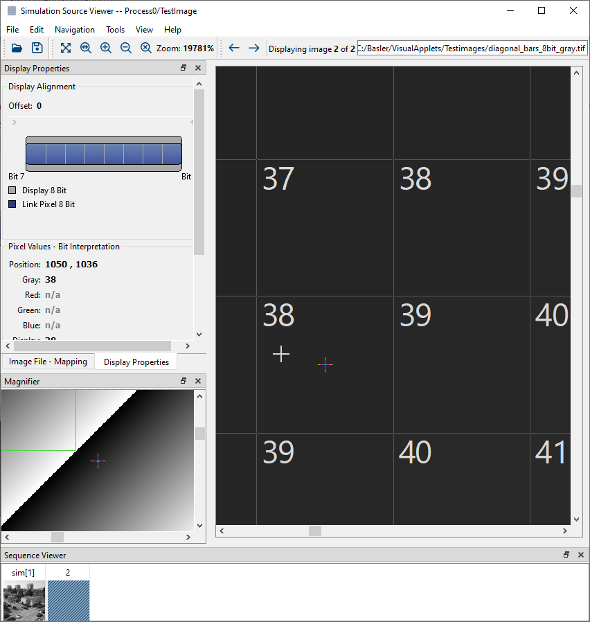
The white/black crosshair cursor shows the position of your mouse cursor.
The colored one is positioned in the center of the pixel the mouse cursor points to. This crosshair cursor is also displayed in the on exactly the same pixel.
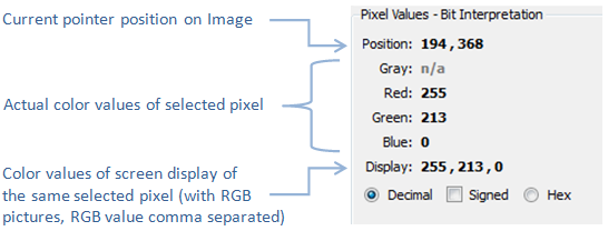
In the settings panel tab the corresponding pixel values are displayed:
You can choose whether you want to see the pixel values as decimal unsigned, decimal signed or hex figures.
shows the value(s) displayed on your screen. This value/these values might be different from the actual color values (or gray value) if a 16 bit or 48 bit image is loaded to your source, since on screen, only 8 bit can be displayed per color channel.
In the tab , you find a table with the image dimensions of the current image (as it is loaded from file) on the left hand side and the image dimensions of the link on the right hand side:
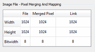
The column is described at 'Pixel Spitting and Merging'.
If an image file has a dimension smaller than the dimension of the link, the image is transferred onto the link on the scale 1:1.
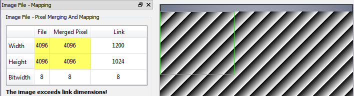
If the image file has a dimension that exceeds the dimension of the link, only part of the picture is used for simulation. You can see in the display panel in the green rectangle which picture part is going to be used for simulation. Also, the corresponding values are highlighted in yellow:
|
提示 |
|---|---|
|
If you cannot see the green rectangle in your display screen, set your viewing options to → . |
In the tab , you also find information on the bit width of your test image (file) and on the bit width of the link the source is connected to:
The column is described at 'Pixel Spitting and Merging'.
If you want to load an image that has a bit width higher than that of the link, you can choose which bits of your image you want to use for simulation. You can make your selection by using a slider:
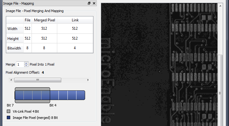
The bit width of the selection slider is the same as the bit width of the link. With the slider you can define a new position for the offset. The offset is the starting point of your bit selection on the bit width of your image. Based on these settings, the immediately calculates the altered image and displays it in the display panel. In the screen shot above, the 4 upper bits have been chosen out of the 8 bit of the 8-bit image. Thus, the test image used for the simulation will only have 16 instead of 256 gray-scale values.
|
Visualization of Altered Test Image in the |
|---|---|
|
Since the display on PC monitors is based on 8-bit information per pixel, an image with only 16 gray-scale values cannot be displayed properly. Thus, for visualization on screen the 16 gray-scale values of the test image are mapped to the 256 gray-scale values of the 8-bit monitor display. This mapping doesn’t change the number of shades of gray displayed (16), but enhances the contrast between them (0 = black, 15 = white). |
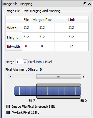
If you, on the contrary, load an image that has a smaller bit width than the link it is loaded on (i.e. the source module is connected to), you can use the same slider in tab to define an offset for the bits of the image on the bit width of the link. The remaining bits of the link are set to NULL.
The picture below shows an example where an 8-bit gray-scale image has been loaded onto a link with a bit width of 12 bit:
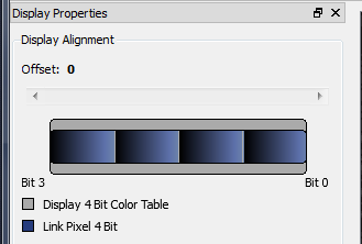
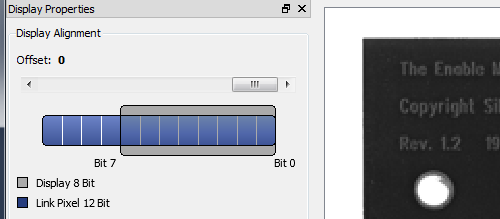
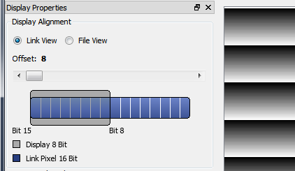
You can define some settings for visualizing the altered test image in the via display alignment:
If the bit width of a link is higher than 8 bit, you have to define which 8 bits out of the link bit width you want to have displayed in the display panel. Since the display on PC monitors is limited to 8 bit per color channel, a higher bit width cannot be displayed.
In the tab , you can define which 8 bits out of the bits of a link you want to have displayed in the display panel. Use the slider to choose the offset for the displayable 8 bits. This display alignment setting has no influence on the simulation.
In the example below, the link has a bit width of 12 bit. With the slider, you can decide which bits out of the 12 you want to have displayed.
The BMP file format allows a maximum of 8 bit per color
channel of a pixel. The TIFF format allows a maximum of 16 bit
per color channel. A higher bit width cannot be simply saved in standard image file
formats.
VisualApplets offers the possibility of pixel splitting to get around these limitations.
To store an image with a high pixel bit width in a standard image file format,
each pixel is split into multiple image file pixels. Thus, it is possible to store
up to 64 bit per color channel in BMP or
TIFF file format, e.g., in 8 x 8-bit pixels. These images
can be viewed in regular image file viewers or image processing programs. Of course,
the VisualApplets generated pixel-split-images will be displayed horizontally
expanded. Thus, in VisualApplets, pixel splitting is a mere storing option for
images with a high bit width (color depth).
To load an image with high bit width that has been stored as a
BMP or TIFF file into your simulation
source, you have to merge the adjacent pixels that share the color information for
one original pixel back to one pixel. Thus, simulation source viewers can merge the
pixel-split-images for correct mapping. The splitting can be done in the
(see 'Evaluating the Simulation Results'). You can define the settings for pixel merge in the tab :
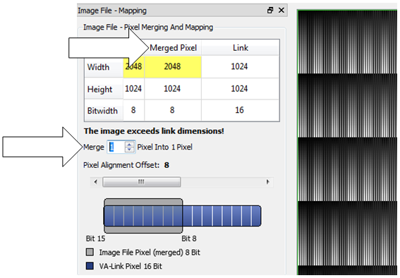
In the following example, a 2048x1024 BMP file with a bit width (color depth)
of 8 bit has been loaded into the source. It is to be interpreted as a 16 bit
1024x1024 image.
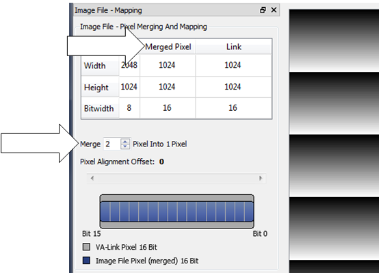
If you enter 2 in the field, the bit width of the image in your source changes from 8 bit to 16 bit per color channel, whereas the row length of the image in your source will be only half as long, thus changing from 2048 to 1024 pixel.
Before merge:
After merge:
After you have loaded a test image or test image sequence to your source and defined all settings for the image, you can start the simulation.
|
Use Simulation Probes |
|---|---|
|
Make sure you inserted (and connected) simulation probes on all positions where you want to check image processing results (see ' Inserting Sources and Probes into your Design'). |
-
From the main menu, select → , or click the toolbar icon
 .
Now, VisualApplets automatically triggers a Design Rules Check 1.
.
Now, VisualApplets automatically triggers a Design Rules Check 1.
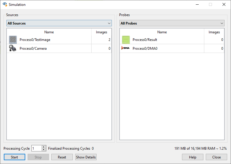
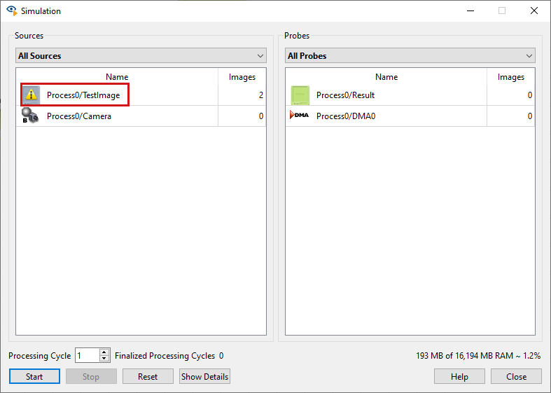
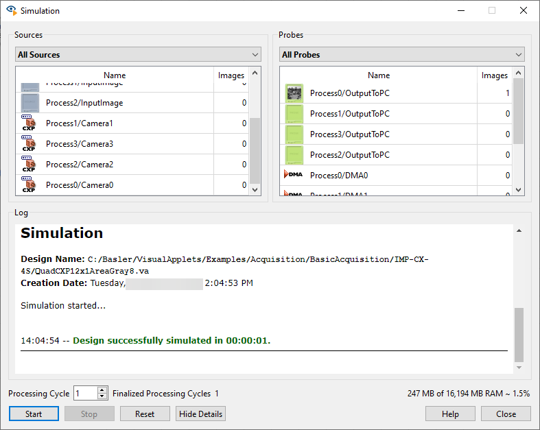
The window opens up:
In the upper pane, all simulation sources and simulation probes currently active in the design are listed. The list serves only information purposes.
In the lower pane of the window, you see the results of Design Rules Check 1.
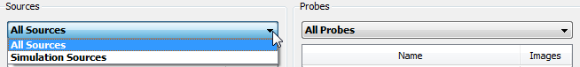
You can change the display of the list via a drop-down list box:
-
and display only the sources and probes you have set for simulation.
-
All Sources and All Probes display all data sources and data destinations within your design.
-
|
Influence of Errors and cautions |
|---|---|
|
A simulation can only be started if no error was detected during Design Rules Check 1. Warnings created by Design Rules Check 1 do not prevent starting the simulation. |
|
Note |
|---|---|
|
Single operators cannot be selected for simulation. A simulation will always run through all operators of a design. |
If the list in the main simulation window shows a simulation source or probe marked by a yellow warning triangle, this source/probe is not connected to a link of your design and will be ignored during simulation.
|
Note |
|---|---|
|
Camera operators do not emit data during simulation. One needs to connect a simulation source to the output link to provide data for the simulation. |
In the field, you can specify how many processing cycles you want the program to carry out.
You can also configure the simulation and the processing cycles via the menu: → → :
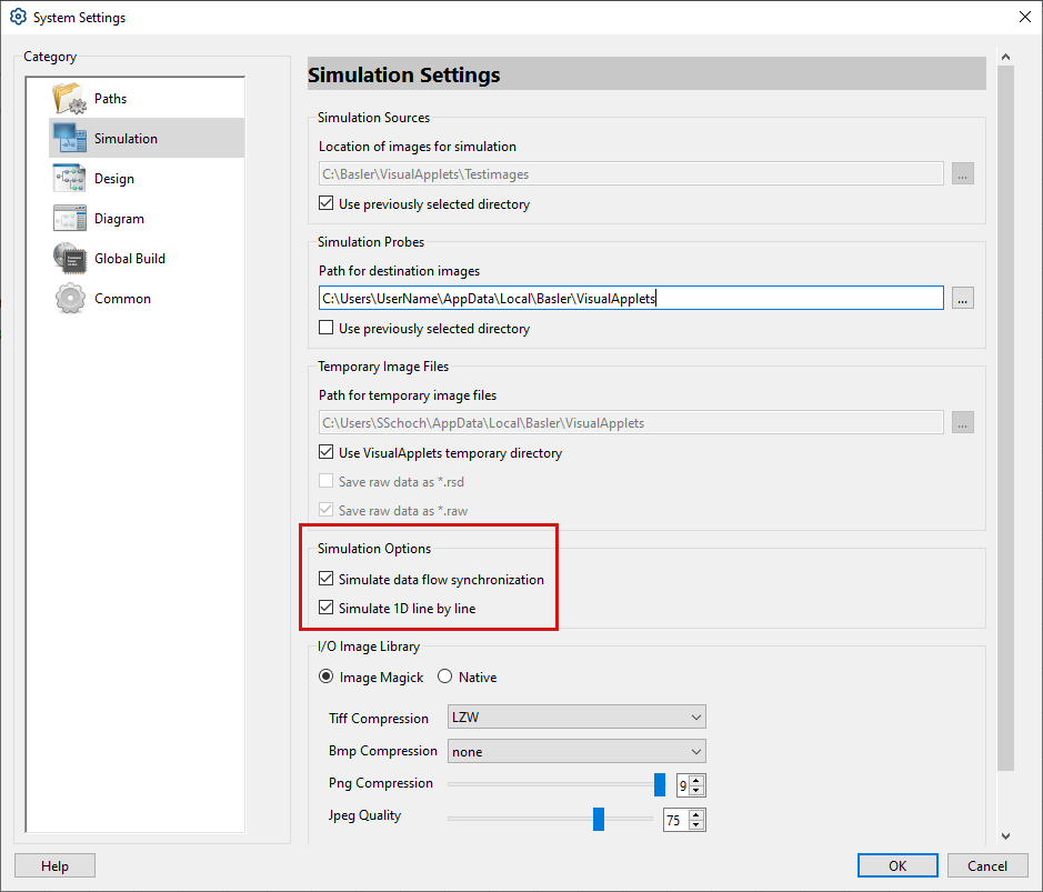
cleared: Each source in your design, e.g. simulation sources and operators like CreateBlankImage, or CoefficientBuffer, emits one data set per cycle. The cycle ends, if no more data is to be processed or transported. A simplified data management allows operators to divert from the behavior of the corresponding entity in hardware. This means, instead of storing incoming data inside the input ports, an operator might implement unrealistically large internal buffers.
selected: The design as a whole is simulated once per cycle from source(s) to sink(s). The focus is on precise modeling of dependencies and accurate data management. Sources are permitted to provide one or more data sets per cycle. The simulation might prevent sources from emitting data if previously generated data is still to be processed. Therefore, operators leave incoming data inside their input ports until data processing requires it to be collected. As long as valid data is stored in the incoming port, upstream operators are prevented from producing data. This causes congestions and corresponds to the concept of inhibits in hardware and allows for the detection of deadlocks.
: 1D data can be processed by aggregating several lines to one 2D frame and simulates it like any other 2D data. This is fast and robust but limits the simulation to exactly one simulation cycle. If you select , each line is processed individually and thus allows multi-step simulations, e.g., to deal with 1D loops. This feature relies on data flow synchronization, this means you can only select this option, if is selected.
|
Behavior of Simulation Probes During |
|---|---|
|
For simulation probes connected to 1D links, incoming line data is appended to the last frame in the simulation probe. After each processing cycle, the respective lines are finalized and a new frame is started. While the simulation dialog is open, the is locked. |
After selecting the desired amount of in the view, the simulation can be run by clicking the button. As the internal status of all operations is maintained, consecutive runs can be launched from the same window, as long as the simulation dialog is kept open. Once the dialog is closed, all operators are reset to their initialization state.
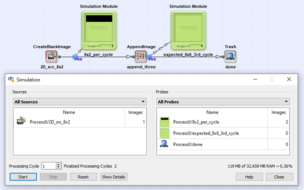
Example: A given AppendImage operator expects three input images for concatenation. A connected source provides one image per processing cycle. The simulation is run for two cycles, a simulation probe connected to the output link of AppendImage does not show any data yet, since AppendImage still lacks one additional image to start the processing.
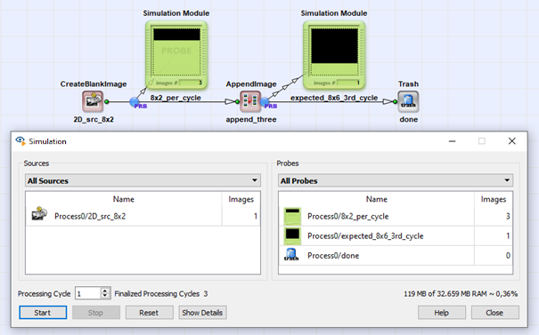
While the simulation dialog is still open, one can perform an additional (third) simulation cycle which in turn provides data at the connected simulation probe.
If the dialog was closed and reopened in the meantime, the additional simulation cycle would be executed after initializing the design and therefore would provide the first of the three required images for AppendImage.
|
Processing Order of Images within a Source Module |
|---|---|
|
In a new processing cycle, always the next image of the image sequence loaded to the source is processed. When all images of the sequence have been processed, the first image of the sequence is processed again. |
If only one image is loaded to the source, this image is processed again and again with each processing cycle. For example, if you specify four processing cycles, the one image of the source is being processed up to four times.
Depending on your design, the number of images fed into the design might differ from the number of images you get as an output, for example when you use the operators SplitImage or RemoveImage. Thus, for one processing cycle, you might get more or less images as result(s) in a probe than you have source modules in your design. See also the example ' Multiple DMA Channel Designs ' in the VisualApplets tutorial.
To clear the simulation and reset it to the start-up condition, use the button.
A reset produces the following effects:
-
The image sequence in all simulation sources is reset, that is, a new simulation will start with the first image of the sequence again.
-
The content of all probes is deleted.
-
All operators are reset to their start-up condition (e.g., image counters, uncollected data in input ports).
Now, you are ready to start the simulation of data processing as defined in your design.
-
Click to start the simulation.
The current simulation status is displayed in a progress bar at the bottom of the Simulation view. Warnings and errors are displayed in the Log panel, which you can open or close by clicking the / button. As soon as warnings or errors occur, the Log panel is displayed automatically.
|
提示 |
|---|---|
|
If you want to, you can keep the viewer windows of your simulation modules open during simulation. However, this will slow down simulation. |
While a simulation is in progress, the simulation probe modules are filled with the resulting images. Thumbnails of the simulation results are displayed in the preview image frames. After opening the simulation viewer window of a simulation probe, the result(s) will be displayed in full size.
|
Automatic Simulation Reset |
|---|---|
|
The simulation will automatically reset when you change your design. On reset, all simulation probes are cleared, too. |
After the simulation, you find the simulation results in the probes.
|
Some Images Are Not Displayed in Probes |
|---|---|
|
When simulation probes contain very large images, VisualApplets may fail to display these images correctly due to memory limitations. In that case, a gray image (i.e. all pixels have the value 205 (0xCD)) is shown. If this happens, use smaller images for your simulation. |
Double-click a probe in your design to open the .
It looks similar to a (see 'Loading the Image File(s) to your Simulation Source(s) '): The settings channel is located at the left hand side, the display channel on the right hand side, and the at the bottom of the window.
In the , you get the simulation results displayed for a first evaluation. You can alter the display options by pixel alignment, and save the images to file. For saving, there are several options available, like, e.g., pixel splitting.
You can zoom in and out on the image displayed in the display channel by either using the corresponding icons in the toolbar, or by using CTRL+MouseWheelUp to zoom in and CTRL+MouseWheelDown to zoom out.
If you choose a very high zooming factor, a pixel grid is displayed for better orientation and the corresponding pixel values are textually represented.
Like in the , on each pixel in the display panel two crosshair cursors are displayed. If you can’t see the two crosshair cursors, zoom in on the picture in the display panel. The white/black crosshair cursor shows the current position of the cursor of your mouse, whereas the colored one is positioned in the center of the pixel the mouse cursor points on. This crosshair cursor is also displayed in the Magnifier on exactly the same pixel.
In the settings panel, the corresponding pixel values are displayed:
You have different options to adjust the interpretation of color values for the selected pixel:
-
You can choose whether you want to see them as hexadecimal numbers or as signed or unsigned decimal numbers.
-
You can set the number of fractional bits for an interpretation as fixed-point numbers.
-
Additionally, you can define a scaling factor which is multiplied to the values. This is useful for performing linear conversions like radiant to degree.
shows the value(s) displayed on your screen. This value/these values might be different from the actual color values (or gray-shade value) if a 16 bit or 48 bit image is in your probe, since on screen, only 8 bit can be displayed per color channel.
You may select a color map which performs tone mapping between the values in Display and the shown color in the image window. This is especially useful when dealing with signed image data or when the contained image characteristics are poorly visible in a grey-scale representation.
If the simulation probe is connected to a link which transports kernels, you can select the individual kernel images in the kernel Row and kernel Column spin boxes in the Kernel panel.
Once an image is simulated, it is instantaneously displayed in the and added to the .
You cannot change the order of images in the .
However, you can delete one or more images of a sequence:
-
Press CTRL and select the images you want to delete.
-
Press DEL or select from the menu → .
If you change the image properties by mapping (for example, when you save 16-bit
images in BMP files), the thumbnails are not refreshed automatically. By default,
the displays the thumbnails of the original simulation results.
VisualApplets is not limited to processing and displaying rectangular images with homogeneous row length. It can also display images with rows that are of different length.
The image size for such images is calculated by VisualApplets as follows:
|
Calculating Image Size for Images with Inhomogeneous Row Lengths |
|---|---|
|
Image size = number of pixels of longest row * number of rows |
Rows with row length NULL are counted as well. The undefined areas of the image are represented in the display by a blue-to-cyan color gradient:
Empty images are displayed by the symbol Empty Image and cannot be saved.

The display panel of the offers two ways of displaying the same image:
-
If you activate Link View, the image is displayed as it looked like when it was passed to the probe by the link.
-
If you activate File View, the image is displayed as it will look when you save it with the current settings to file.
Since monitors always use 8 bit per color channel, images with higher or lower bit width cannot be displayed without further ado.
If a simulation result has a bit width higher than 8 bit, you can use the offset slider to select the 8 bit you want to have displayed in the display panel:
In this example, the upper 8 bits of a 16-bit gray scale are chosen for display.
If the bit width of the image is smaller than 8 bit, the gray-scale values of the test image are automatically mapped to the 256 gray-scale values of the 8-bit monitor display. This mapping doesn’t change the number of shades of gray displayed, but enhances the contrast between them. Without this mapping, the human eye might not be able to see an image at all. Take, for example, 1-bit images: If the values 0 and 1 are used for monitor display without mapping, both are interpreted as black by the human eye. In this case, the automatic bit width mapping of VisualApplets interprets 0 as 0 (black) and 1 as 255 (white).
The view shows the individual color values or gray values of a line. You can open the via the menu .
There are two output areas:
-
: The individual color values or gray values of the entire line are displayed.
-
: Enlarges an area marked in the view. The area that is currently displayed in the view is highlighted in the view with a white background. You can move the area displayed in the view with the scroll bar under the view.
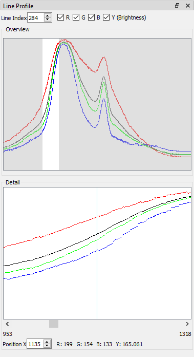
With the spin box , you can select a certain line in the image and the line is marked in the panel.
For color images, you can switch the individual color channels on or off with the checkboxes , , , and . stands for brightness. In addition, you can select a specific pixel position in the line via the spin box or with the cyan marker. To use the cyan marker, just move the mouse into the view. The values are then displayed in , , , and .
The view is a representation of the distribution of color values or gray values only of the selected line in an image. You can open the via the menu .
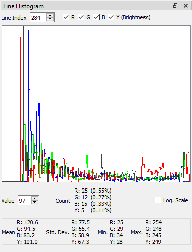
The histogram view is scaled so it always spans the full height of the diagram.
With the spin box , you can select a certain line in the image. As in the view, the line is then marked in the panel.
For color images, you can switch the individual color channels on or off with the checkboxes , , , and . stands for brightness. In addition, you can select a specific color value via the spin box or with the cyan marker. To use the cyan marker, set the mouse cursor into the output view.
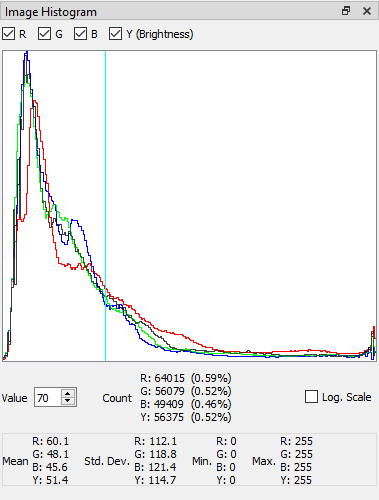
For larger color depths, for example 16-bit images, the spin box is displayed instead of the spin box and the bin ranges are displayed next to it: 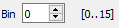
For a selected or number, the number of pixels with values in the corresponding range are shown in . You can manually enter the number in or or select the number by pointing the mouse to the diagram.
For color images, the output is split into the basic color values RGB and the brightness value Y.
The view is a representation of the distribution of color values or gray values in an image. You can open the via the menu .
The histogram view is scaled so it always spans the full height of the diagram.
For color images, you can switch the individual color channels on or off with the checkboxes , , , and . stands for brightness. In addition, you can select a specific color value via the spin box or with the cyan marker. To use the cyan marker, set the mouse cursor into the output view.
For larger color depths, for example 16-bit images, the spin box is displayed instead of the spin box and the bin ranges are displayed next to it:
For a selected or number, the number of pixels with values in the corresponding range are shown in . You can manually enter the number in or or select the number by pointing the mouse to the diagram.
For color images, the output is split into the basic color values RGB and the brightness value Y.
You can save your simulation results in the image file formats TIFF/TIF, BMP, JPEG/JPG, PNG, GIF, and PSD. The TIFF format offers native support of 8 and 16 bit per color channel, BMP offers only 8 bit per channel.
Before you actually save your image as TIFF/TIF or BMP file, you should define all saving settings in the Save Options dialog.
-
To open the dialog, from the main menu of the select → . As a result, the panel opens up on the right hand side of the .
In Destination File Format, you can define the format in which you want to save the image:
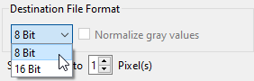
If you want to save a 1-bit simulation result in an 8-bit file format, check the box Normalize gray values. Normalizing in this context means mapping 0 to 0 (black) and 1 to 255 (white).
If the bit width of the image (= the bit width of the link) is the same as the bit width of the file format you have chosen for saving, you can save the image 1:1.
If the bit width of the image is smaller than the bit width of the file
format, you can change the pixel alignment offset using the slider.
This way, you can save the bits of the simulation result on a certain location
within the (larger) pixel of the file format. For example, save
the bits of a 12-bit link on the lowest 12 bits or the highest 12 bits of a 16 bit
TIFF image.
If the bit width of the image is larger than the bit width of the file format, you can use the slider for choosing which bits out of an image pixel you want to save to file and which bits can be discarded.
To get a preview on the (stripped) image as it will be saved to file: In the main window of the Simulation Probe Viewer, set the radio button on top of the settings panel to File View.
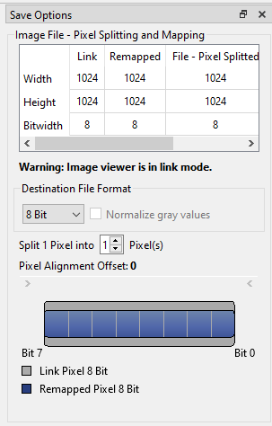
If you want to use the pixel splitting option of VisualApplets, you can define to how many pixels you want to split the color information of one pixel (see also 'Pixel Spitting and Merging') .
If you want to save, for example, a 16-bit simulation result in a 8-bit BMP file,
set Split 1 Pixel into to 2 pixels. Now, the 16-bit pixel of
the image is split into two 8-bit pixels.
By splitting, the row length is doubled, tripled, etc. (depending on the splitting factor). In our example, the row length is doubled. Regular image visualization/processing programs can display these split images. But since they assume a bit width of 8 bit, the image display is expanded horizontally.
|
Reconversion of Split Image |
|---|---|
|
You can load a split image in a simulation source and re-convert it to its original bit width by using the pixel merge option (see 'Pixel Spitting and Merging'). |
![[Important]](../common/images/admon/important.png) |
Important |
|---|---|
|
When selecting → from the main menu, all settings you have defined in the Save Options dialog are applied. |
For saving your simulation results to file, proceed as follows:
-
Select from the main menu → .
-
Define saving location and file name.
-
Click .
|
Saving an Image Sequence |
|---|---|
|
You can also save a whole image sequence. To save an image sequence, select all images you want to save in the Simulation Viewer. To do so, hold CTRL pressed and click on the images. Then, select from the main menu → . The saved images are automatically numbered. |
Q: I converted a color image to a gray-scale image and tried loading it to a simulation source. However, VisualApplets denies loading the image onto a one-channel link. What is the problem?
A: The image still uses 3 channels (with 0% saturation) for color information. Just convert your image to a one-channel image.
Q: My simulation probes do not include any results after simulation. What is the problem?
A: You might not have simulated enough simulation cycles. Increase the number of cycles. Moreover, your algorithm might not generate any output images. Check the respective operator restrictions in the operator references. Also, simulation probes connected to signal links never show output data.
Q: My simulation probes are cleared automatically. Why?
A: Each time the design is modified, the simulation probes might get cleared. This does not occur for minor changes of your design like moving modules or modifying internal parameters of operators that do not affect current ports. Probes are invalidated for changes that alter the topology of the design or parameter changes that are propagated through links to connected operators.
